Usage and Examples
GWAS SVatalog provides two ways to obtain the end goal of fine-mapping GWAS loci using structural vairants.
Choosing a genomic region of interest
Selecting a phenotype of interest with/without a specific loci
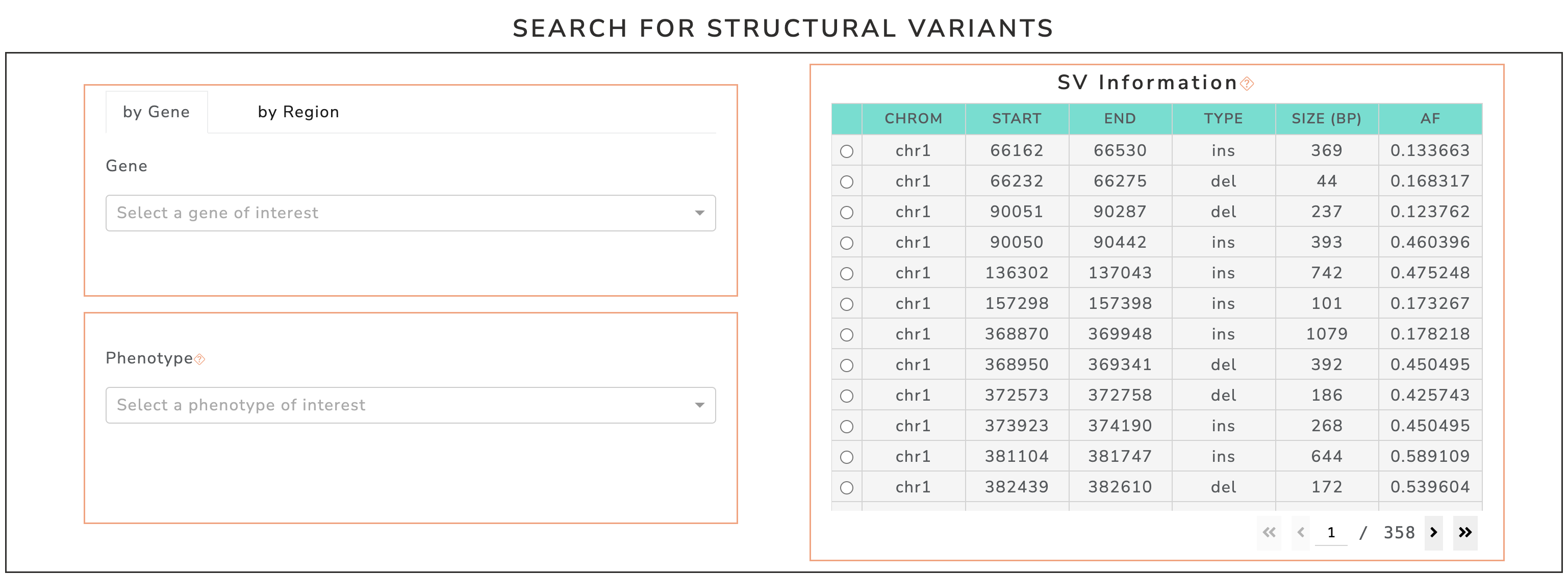
Screenshot of filter section availible to subset SV list in GWAS SVatalog.
1. Genomic Region
This method subsets the list of structural variants solely by the genomic region of interest.
Selecting by Coordinates
Simply selecting chromosome of interest and/or entering the desired range.
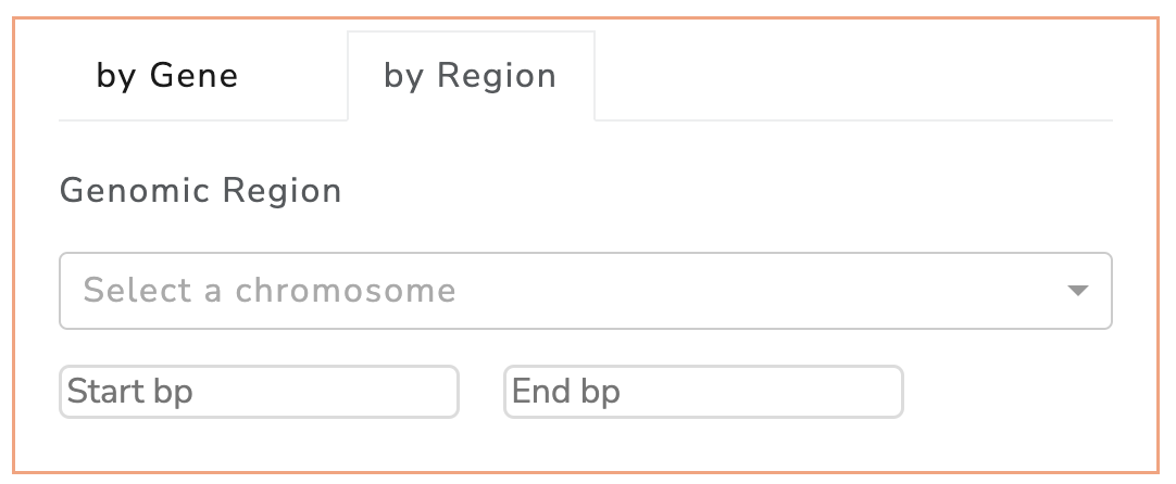
Screenshot of genomic region filter in GWAS SVatalog.
Selecting by Gene
When selecting a gene of interest, the SVs displayed are within 100kb of the start and end of the gene chosen.
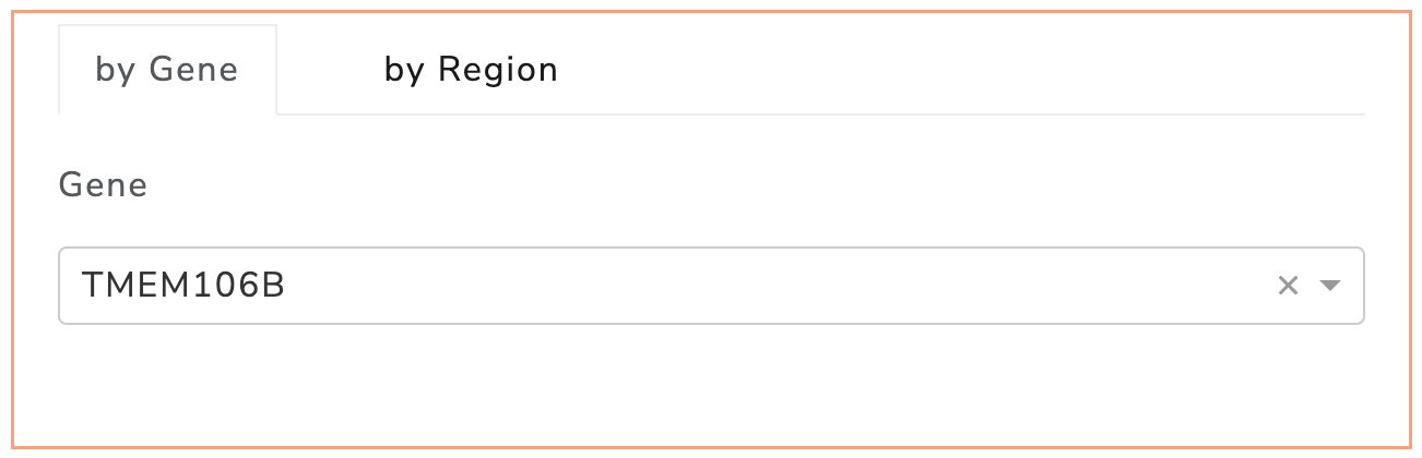
Screenshot of gene filter in GWAS SVatalog.
Selecting an SV
The 35,732 structural variants in this table are subsetted by the filters applied. Each row is a unique SV with MAF ≥ 0.1.
Select a SV to analyze further.
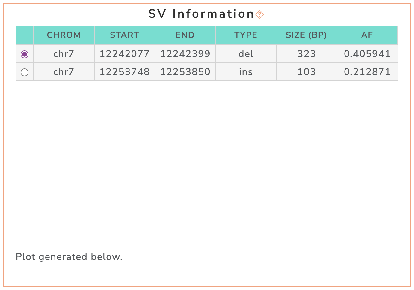
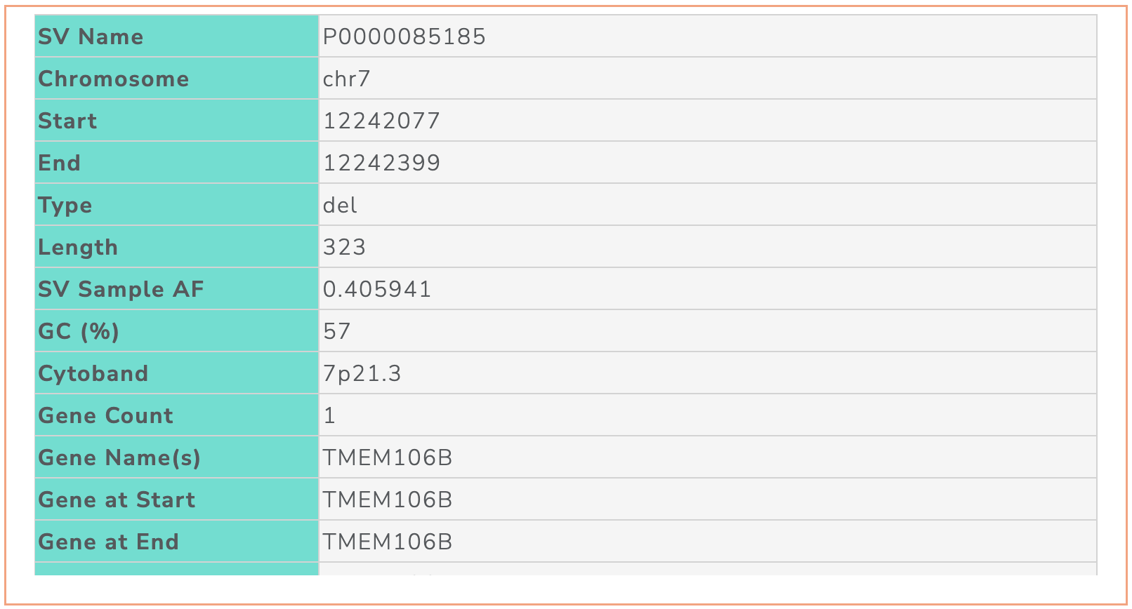
Screenshot of the SV information table in GWAS SVatalog.
SV Annotations
Annotations generated for the selected SV are displayed here. This document explains the meaning of each column in detail.
Screenshot of the SV annotation table in GWAS SVatalog.
Interactive Plot
The visualization shows the selected SV and linkage disequilibrium statistics (D’/r2) for SNPs within 1 Mb of its boundries. These SNPs are significant with genome-wide association studies studies as depicted in GWAS Catalog. Each marker is a unique SNP where the hover label shows information on one entry in GWAS Catalog. When a SNP is clicked, a table below populates with additional information (see SNP Table).
The default LD statistic is D’, the toggle can be used to visualize r2 on the y axis if required.
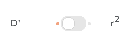
Screenshot of D’ to r2 toggle button for the interactive plot in GWAS SVatalog.
The representative transcript for each gene obtained from MANE are shown in the plot. The direction of the arrow beside each gene name represents the direction of the transcript. The user can additionally download information of the SNPs shown in the plot as a .csv file when clicking the “Export SNP Data to CSV” button to the right of the visualziation. See SNP Table for column descriptions.
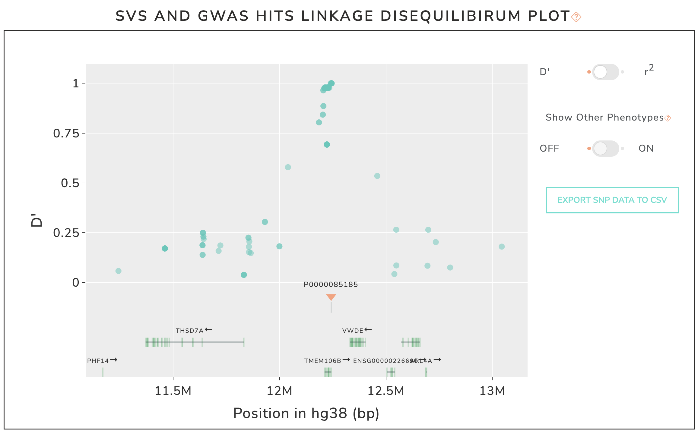
Screenshot of interactive plot in GWAS SVatalog.
SNP Table
This table is populated based on the SNP selected in the plot. The SNP information is a combination of GWAS Catalog entries and linkage disequilibrium statistics for the selected SV.
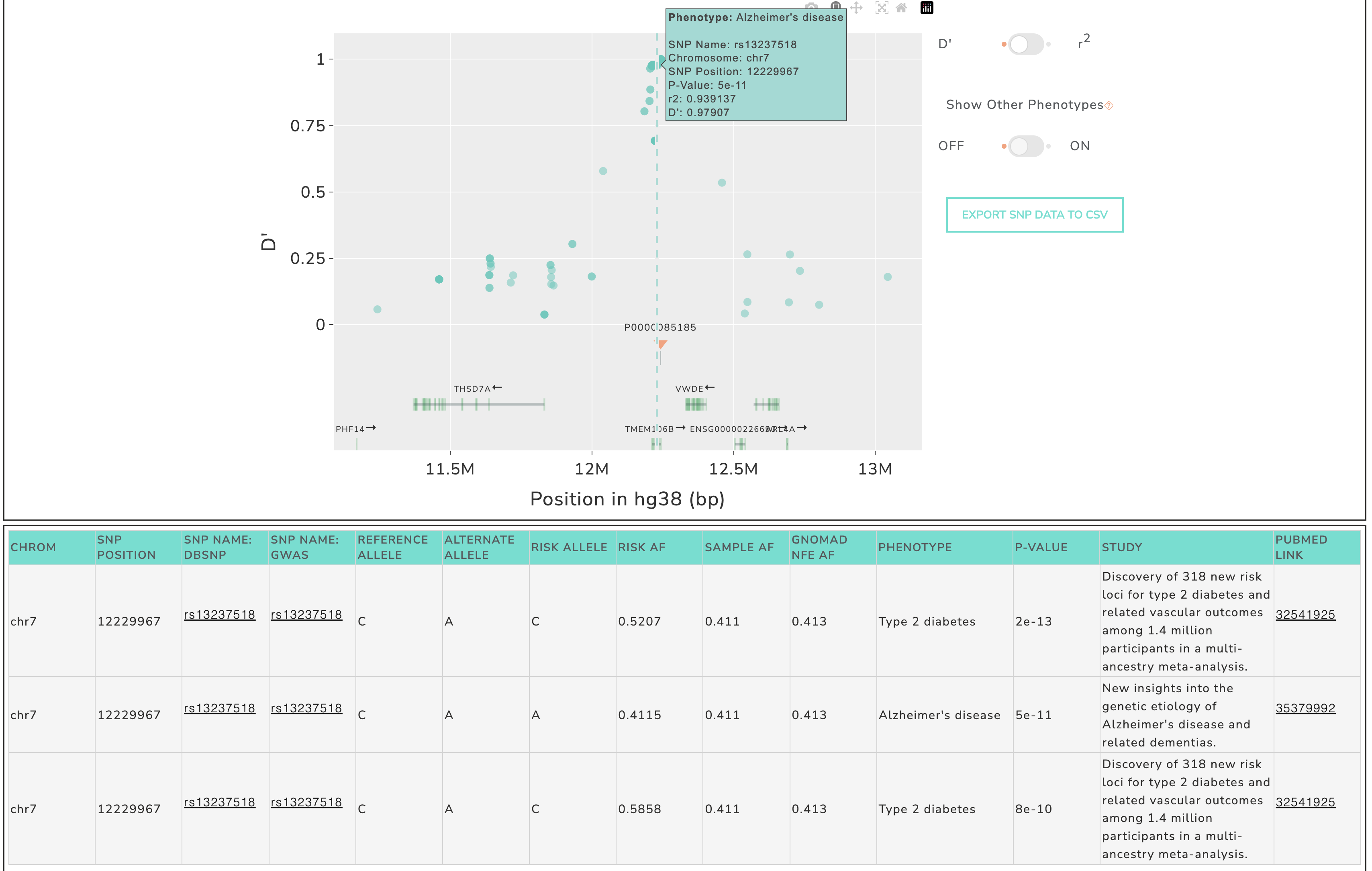
Screenshot example of selecting a SNP in the plot and populating the SNP table in GWAS SVatalog.
Description of columns seen in the table:
Chromosome: chromosome number
SNP Position: base pair location on chromosome (hg38 coordinates)
SNP Name: dbSNP: rsID from dbSNP
SNP Name: GWAS: rsID from the GWAS Catalog entry
Reference Allele: reference allele from hg38
Alternate Allele: alternate allele
Risk Allele: risk allele provided by GWAS Catalog
Risk AF: risk allele frequency provided by GWAS Catalog
Sample AF: allele frequnency from 101 sample cohort (insert citation of paper)
gnomAD NFE AF: alelle frequency provided by gnomAD for the Non-Finnish European population
Phenotype: disease/trait provided by GWAS Catalog
P-Value: statistic provided by GWAS Catalog
Study: name of the study from which this entry is derived
Pubmed Link: PubMed link to the research paper for this entry
Additional columns in the download file:
SV Name: name of the structural variant
SV Start: start base pair location
SV End: end base pair location
SV Type: type of indel (insertion, deletion, duplication or inversion)
SV AF: allele frequency of the SV from the samples used during calculation (insert citation of paper)
r2: LD statistic - square of the correlation coefficient between the SV and SNP
D’: LD statistic - measure of predictability of the SV and SNP based on one another
P-Value_log10: log10 of the statistic provided by GWAS Catalog
2. Phenotype
This method subsets the list of structural variants by the phenotype of interest. These SVs have linkage disequilibrium statistics with at least one GWAS-significant SNP for the selected phenotype.
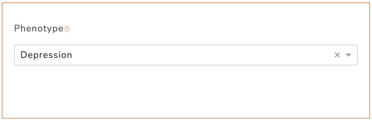
Selecting by Phenotype
The list of phenotypes have been obtained from GWAS Catalog.
Screenshot of phenotype filter in GWAS SVatalog.
Selecting by Genomic Loci
In addition to selecting a phenotype, the user can optionally subset the list of SVs further by choosing a genomic region or gene of interest (see Selecting by Coordinates and Selecting by Gene).
Selecting an SV
SV Annotations
Interactive Plot
The visualization shows the selected SV and p-value of GWAS-associated SNPs for the chosen phenotype. These SNPs are significant with genome-wide association studies studies as depicted in GWAS Catalog. The color of each SNP marker is based on the D’ statistic with the selected SV. The user has an option to switch the color to depict r2 instead by clicking the toggle to the right.
Screenshot of D’ to r2 toggle button for the interactive plot in GWAS SVatalog.
The user also has an option to visualize p-value for SNPs from other phenotypes within 100 kb of the current region. The linkage disequilibrium statistics (D’/r2) between each of these SNPs and the selected SV will be displayed in the hover label.
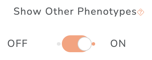
Screenshot of show other phenotype toggle button for the interactive plot in GWAS SVatalog.
The representative transcript for each gene obtained from MANE are shown in the plot. The direction of the arrow beside each gene name represents the direction of the transcript. The user can additionally download information of the SNPs shown in the plot as a .csv file when clicking the “Export SNP Data to CSV” button to the right of the visualziation. See SNP Table for column descriptions.
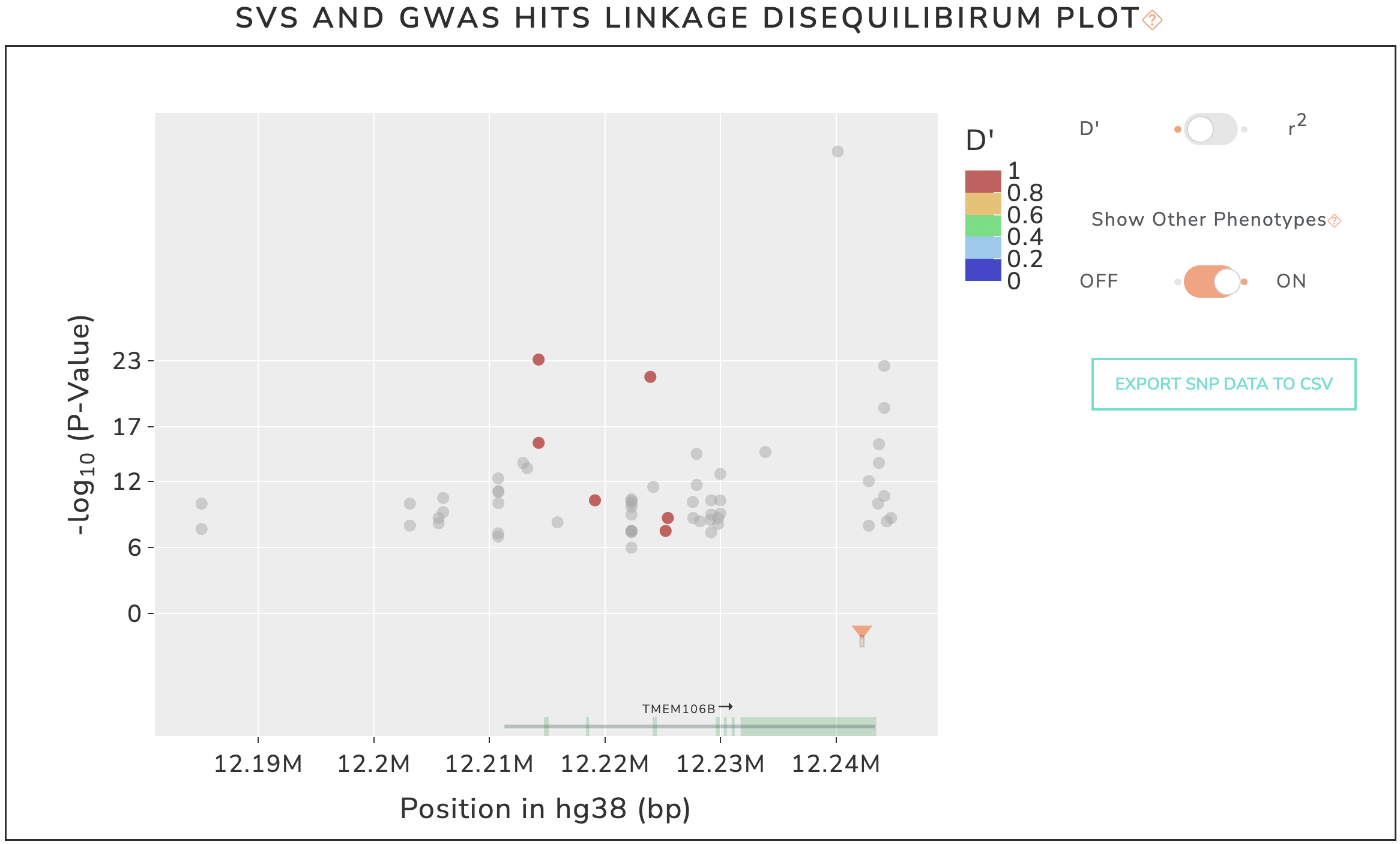
Screenshot of interactive plot after selecting a specific phenotype in GWAS SVatalog.